3. Decision Tree : 의사 결정 나무
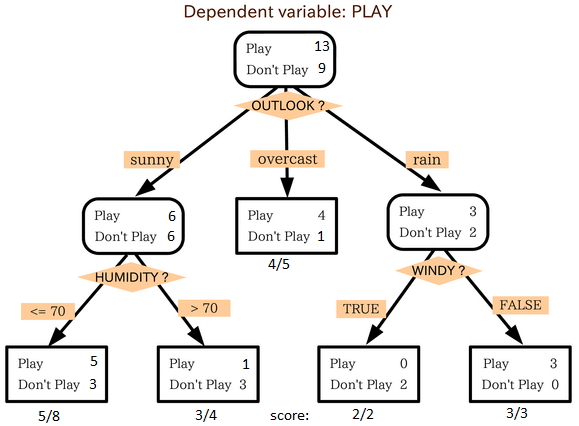
This is one of my favorite algorithm and I use it quite frequently. It is a type of supervised learning algorithm that is mostly used for classification problems. Surprisingly, it works for both categorical and continuous dependent variables. In this algorithm, we split the population into two or more homogeneous sets. This is done based on most significant attributes/ independent variables to make as distinct groups as possible. For more details, you can read: Decision Tree Simplified.
source: statsexchange
입력변수가 여러개다. (맑음, 보통, 비온다) - (습도가 높다/낮다) - (바람이 분다/안분다)
이로부터 야구 경기를 할지 말지 예측(출력) 하는 것. test set으로부터 어떻게 입력변수로 분기시키면 최적의 예측(classification)이 가능한지 모델을 만든다.
In the image above, you can see that population is classified into four different groups based on multiple attributes to identify ‘if they will play or not’. To split the population into different heterogeneous groups, it uses various techniques like Gini, Information Gain, Chi-square, entropy.
어떻게 의사결정 나무가 모델링되는 지는 여러가지 방법이 있고 여기서는 몰라도 된다.
The best way to understand how decision tree works, is to play Jezzball – a classic game from Microsoft (image below). Essentially, you have a room with moving walls and you need to create walls such that maximum area gets cleared off with out the balls.
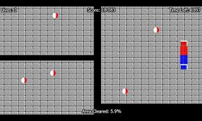
So, every time you split the room with a wall, you are trying to create 2 different populations with in the same room. Decision trees work in very similar fashion by dividing a population in as different groups as possible.
More: Simplified Version of Decision Tree Algorithms
Python Code
#Import Library
#Import other necessary libraries like pandas, numpy...
from sklearn import tree
#Assumed you have, X (predictor) and Y (target) for training data set and x_test(predictor) of test_dataset
# Create tree object
model = tree.DecisionTreeClassifier(criterion='gini') # for classification, here you can change the algorithm as gini or entropy (information gain) by default it is gini
# model = tree.DecisionTreeRegressor() for regression
# Train the model using the training sets and check score
model.fit(X, y)
model.score(X, y)
#Predict Output
predicted= model.predict(x_test)
R Code
library(rpart)
x <- cbind(x_train,y_train)
# grow tree
fit <- rpart(y_train ~ ., data = x,method="class") # 입력변수에 분기에 활용할수 있는 조건이 들어 있다
summary(fit)
#Predict Output
predicted= predict(fit,x_test)
4. SVM (Support Vector Machine)
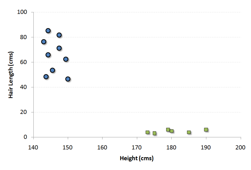
It is a classification method. In this algorithm, we plot each data item as a point in n-dimensional space (where n is number of features you have) with the value of each feature being the value of a particular coordinate.
For example, if we only had two features like Height and Hair length of an individual, we’d first plot these two variables in two dimensional space where each point has two co-ordinates (these co-ordinates are known as Support Vectors)
N차원 공간에 이미 분류된(서로 다른 색깔의) 공을 나누는 직선을 긋는 것이다.
Now, we will find some line that splits the data between the two differently classified groups of data. This will be the line such that the distances from the closest point in each of the two groups will be farthest away.
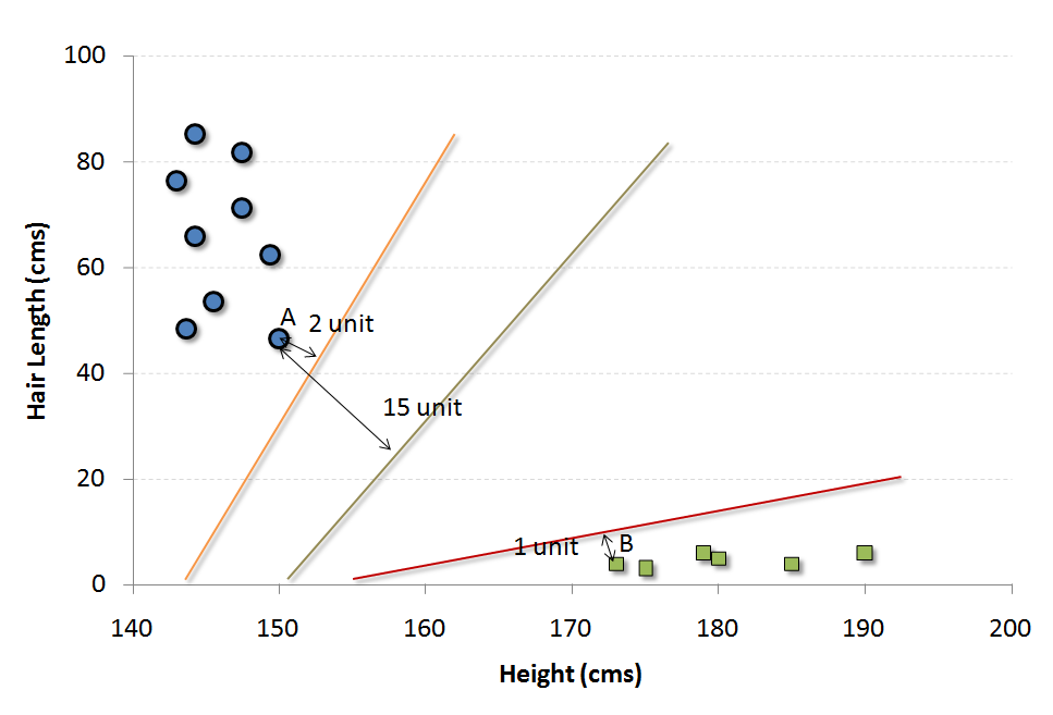
In the example shown above, the line which splits the data into two differently classified groups is the black line, since the two closest points are the farthest apart from the line. This line is our classifier. Then, depending on where the testing data lands on either side of the line, that’s what class we can classify the new data as.
More: Simplified Version of Support Vector Machine
Think of this algorithm as playing JezzBall in n-dimensional space. The tweaks in the game are:
- You can draw lines / planes at any angles (rather than just horizontal or vertical as in classic game)
- The objective of the game is to segregate balls of different colors in different rooms.
- And the balls are not moving.
Python Code
#Import Library
from sklearn import svm
#Assumed you have, X (predictor) and Y (target) for training data set and x_test(predictor) of test_dataset
# Create SVM classification object
model = svm.svc() # there is various option associated with it, this is simple for classification. You can refer link, for mo# re detail.
# Train the model using the training sets and check score
model.fit(X, y)
model.score(X, y)
#Predict Output
predicted= model.predict(x_test)
R Code
library(e1071)
x <- cbind(x_train,y_train)
# Fitting model
fit <-svm(y_train ~ ., data = x)
summary(fit)
#Predict Output
predicted= predict(fit,x_test)
'Machine Learning & Data Mining' 카테고리의 다른 글
| Essentials of Machine Learning Algorithms #5. K-Means, Random Forest (0) | 2015.09.26 |
|---|---|
| Essentials of Machine Learning Algorithms #4. Navie Bayes, KNN (0) | 2015.09.26 |
| Essentials of Machine Learning Algorithms #2 Linear and Logistic Regression (0) | 2015.09.26 |
| Essentials of Machine Learning Algorithms #1 Intro (0) | 2015.09.26 |
| Deep Learning Tutorial (0) | 2015.09.22 |
