1. Linear Regression
It is used to estimate real values (cost of houses, number of calls, total sales etc.) based on continuous variable(s). Here, we establish relationship between independent and dependent variables by fitting a best line. This best fit line is known as regression line and represented by a linear equation Y= a *X + b.
The best way to understand linear regression is to relive this experience of childhood. Let us say, you ask a child in fifth grade to arrange people in his class by increasing order of weight, without asking them their weights! What do you think the child will do? He / she would likely look (visually analyze) at the height and build of people and arrange them using a combination of these visible parameters. This is linear regression in real life! The child has actually figured out that height and build would be correlated to the weight by a relationship, which looks like the equation above.
초등학교 키(입력), 몸무게(목표) Data가 있다. 여기서 키만 가지고 몸무게를 추정하는 1차 함수를 만들고, 이의 결과 예측 수준을 최대로 높인다. 이로써 키만가지고 몸무게를 예측할수 있게 된다. 여기서 입력이 늘어나면 Multiple되고, Curvilinear도 될수 있다.
In this equation:
- Y – Dependent Variable
- a – Slope
- X – Independent variable
- b – Intercept
These coefficients a and b are derived based on minimizing the sum of squared difference of distance between data points and regression line.
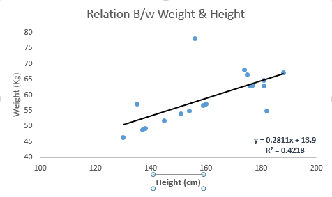
Look at the below example. Here we have identified the best fit line having linear equationy=0.2811x+13.9. Now using this equation, we can find the weight, knowing the height of a person.
Linear Regression is of mainly two types: Simple Linear Regression and Multiple Linear Regression. Simple Linear Regression is characterized by one independent variable. And, Multiple Linear Regression(as the name suggests) is characterized by multiple (more than 1) independent variables. While finding best fit line, you can fit a polynomial(다항) or curvilinear(곡선) regression. And these are known as polynomial or curvilinear regression.
Python Code
#Import Library
#Import other necessary libraries like pandas, numpy...
from sklearn import linear_model
#Load Train and Test datasets
#Identify feature and response variable(s) and values must be numeric and numpy arrays
x_train=input_variables_values_training_datasets
y_train=target_variables_values_training_datasets
x_test=input_variables_values_test_datasets
# Create linear regression object
linear = linear_model.LinearRegression()
# Train the model using the training sets and check score
linear.fit(x_train, y_train)
linear.score(x_train, y_train)
#Equation coefficient and Intercept
print('Coefficient: \n', linear.coef_)
print('Intercept: \n', linear.intercept_)
#Predict Output
predicted= linear.predict(x_test)
R Code
#Load Train and Test datasets
#Identify feature and response variable(s) and values must be numeric and numpy arrays
x_train <- input_variables_values_training_datasets ## (훈련, 몸무게 입력치)
y_train <- target_variables_values_training_datasets ## (훈련, 키 목표치)
x_test <- input_variables_values_test_datasets ## (테스트, 몸무게 입력치)
x <- cbind(x_train,y_train)  ## 훈련셋으로 묶는다
# Train the model using the training sets and check score
linear <- lm(y_train ~ ., data = x)  ## x셋으로부터 목표치(몸무게)를 만드는 회귀모델을 만드다.
summary(linear)        ## 만들어진 회수함수를 요약해서 보여준다.
#Predict Output
predicted= predict(linear,x_test) ## 테스트 입력치를 통해 목표치를 출력한다.
2. Logistic Regression
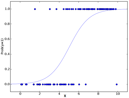
Don’t get confused by its name! It is a classification not a regression algorithm. It is used to estimate discrete values ( Binary values like 0/1, yes/no, true/false ) based on given set of independent variable(s). In simple words, it predicts the probability of occurrence of an event by fitting data to a logit function. Hence, it is also known as logit regression. Since, it predicts the probability, its output values lies between 0 and 1 (as expected).
회권분석같지만 사실상 classification(분류)다. 입력- 출력에서 출력은 yes/no에 대한 확률값으로 나타난다.
키를 입력값으로 농구부에 입단할 가능성을 출력값으로 한다.
Again, let us try and understand this through a simple example.
Let’s say your friend gives you a puzzle to solve. There are only 2 outcome scenarios – either you solve it or you don’t. Now imagine, that you are being given wide range of puzzles / quizzes in an attempt to understand which subjects you are good at. The outcome to this study would be something like this – if you are given a trignometry based tenth grade problem, you are 70% likely to solve it. On the other hand, if it is grade fifth history question, the probability of getting an answer is only 30%. This is what Logistic Regression provides you.
입력: 고2 미적분 --> 출력: 풀수 있는 확률 25%
입력: 중2 인수분해 --> 출력: 풀수 있는 확률 85%
Coming to the math, the log odds of the outcome is modeled as a linear combination of the predictor variables.
odds= p/ (1-p) = probability of event occurrence / probability of not e. occur. p=70% --> 233.3%
ln(odds) = ln(p/(1-p))
logit(p) = ln(p/(1-p)) = b0+b1X1+b2X2+b3X3....+bkXk
Above, p is the probability of presence of the characteristic of interest. It chooses parameters that maximize the likelihood of observing the sample values rather than that minimize the sum of squared errors (like in ordinary regression).
로지스틱스 회귀 모델은 S.E.의 sum을 줄이기 보다는 결과를 맞출 확률을 최대화하는 쪽으로 변수를 선택한다.
Now, you may ask, why take a log? For the sake of simplicity, let’s just say that this is one of the best mathematical way to replicate a step function. I can go in more details, but that will beat the purpose of this article.
로그값을 쓰는 이유는 이것이 Step Function(계단식 함수) 을 모사하기에 가장 좋은 방법이기 때문이다. 아마도 가운데 grey한 구간이 아닌 양쪽끝 (0 또는 1)에 값이 몰리기 때문으로 보임
 Python Code
#Import Library
from sklearn.linear_model import LogisticRegression
#Assumed you have, X (predictor) and Y (target) for training data set and x_test(predictor) of test_dataset
# Create logistic regression object
model = LogisticRegression()
# Train the model using the training sets and check score
model.fit(X, y)
model.score(X, y)
#Equation coefficient and Intercept
print('Coefficient: \n', model.coef_)
print('Intercept: \n', model.intercept_)
#Predict Output
predicted= model.predict(x_test)
R Code
x <- cbind(x_train,y_train)
# Train the model using the training sets and check score
logistic <- glm(y_train ~ ., data = x,family='binomial') # x학습셋으로부터 결과값인 확률(y)를 추정할수 있는
summary(logistic)                                        # 함수를 만든다.
#Predict Output
predicted= predict(logistic,x_test)
Furthermore..
There are many different steps that could be tried in order to improve the model:
- including interaction terms
- removing features
- regularization techniques
- using a non-linear model
'Machine Learning & Data Mining' 카테고리의 다른 글
| Essentials of Machine Learning Algorithms #4. Navie Bayes, KNN (0) | 2015.09.26 |
|---|---|
| Essentials of Machine Learning Algorithms #3. Decision Tree & SVM (0) | 2015.09.26 |
| Essentials of Machine Learning Algorithms #1 Intro (0) | 2015.09.26 |
| Deep Learning Tutorial (0) | 2015.09.22 |
| Deep learning 기반 T map POI 추천 기술개발 사례 (0) | 2015.09.22 |
