5. Naive Bayes 나이브 베이즈 모델
It is a classification technique based on Bayes’ theorem with an assumption of independence between predictors. In simple terms, a Naive Bayes classifier assumes that the presence of a particular feature in a class is unrelated to the presence of any other feature. For example, a fruit may be considered to be an apple if it is red, round, and about 3 inches in diameter. Even if these features depend on each other or upon the existence of the other features, a naive Bayes classifier would consider all of these properties to independently contribute to the probability that this fruit is an apple.
나이브 베이즈 모델은 입력변수가 서로 독립이라고 가정한다.
예들들어 5년내 당뇨병 발병 가능성을 예측할 때 입력변수로 현재 몸무게, 평소운동량, 음주/흡연량, 설탕소비량을 입력값으로 쓴다고 가정해보자. 그런데 나이브 베이즈 모델은 설탕 소비량, 평소 운동량이 몸무게에 아무런 영향을 주지 않는다고 가정한다.
이름처럼 나이브한 구석이 있다.
Naive Bayesian model is easy to build and particularly useful for very large data sets. Along with simplicity, Naive Bayes is known to outperform even highly sophisticated classification methods.
대용량 데이터에 적용하기 좋고, 다른 분류(Classification) 보다 성능이 좋다.
Bayes theorem provides a way of calculating posterior probability P(c|x) from P(c), P(x) and P(x|c). Look at the equation below:
P(c|x) = 비만인 경우 당뇨가 될 확률 (= posterior probability)
P(x|c) = 당뇨인 경우 비만인 확률(=likelihood) , P(x) = 전체중 비만일 확률, P(c) = 전체 중 당뇨인 확률(=prior probability)
|
c 당뇨 Y | 당뇨 N | 계 |
|
x 비만 Y |
3 |
17 | 20 P(x) = 20% | P(c|x) = 15% = 3/20 모른다 가정 |
비만 N |
2 |
78 | 80 |
|
계 | 5 P(c) = 5% | 95 | 100 |
|
| P(x|c) = 60% = 3/5 |
|
|
|
P(c|x) = 15% = 3/20 = 60% * 5% /20%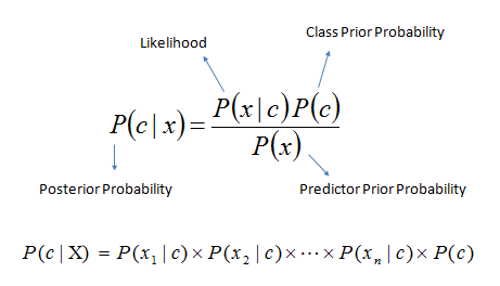
Here,
- P(c|x) is the posterior probability of class (target) given predictor (attribute).
- P(c) is the prior probability of class.
- P(x|c) is the likelihood which is the probability of predictor given class.
- P(x) is the prior probability of predictor.
Example: Let’s understand it using an example. Below I have a training data set of weather and corresponding target variable ‘Play’. Now, we need to classify whether players will play or not based on weather condition. Let’s follow the below steps to perform it.
Step 1: Convert the data set to frequency table
Step 2: Create Likelihood table by finding the probabilities like Overcast probability = 0.29 and probability of playing is 0.64.
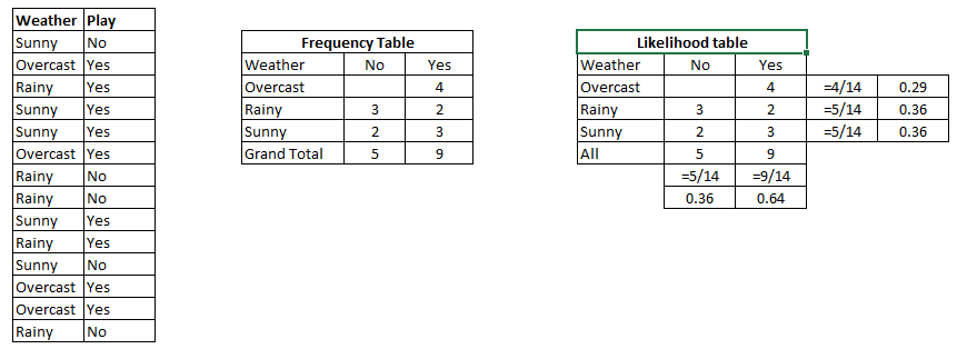
Step 3: Now, use Naive Bayesian equation to calculate the posterior probability for each class. The class with the highest posterior probability is the outcome of prediction.
Problem: Players will pay if weather is sunny, is this statement is correct?
We can solve it using above discussed method, so P(Yes | Sunny) = P( Sunny | Yes) * P(Yes) / P (Sunny)
Here we have P (Sunny |Yes) = 3/9 = 0.33, P(Sunny) = 5/14 = 0.36, P( Yes)= 9/14 = 0.64
Now, P (Yes | Sunny) = 0.33 * 0.64 / 0.36 = 0.60, which has higher probability.
위 표의 경우 3/5 = 60%하는 P(Yes/Sunny) 값이 금방 나오지만, 현실 사례에서는 그렇지 않기 때문에 Navie Bayse를 사용
Decision tree와 달리 하나의 값(Sunny)만으로도 결과(yes)확률을 알수 있다
Naive Bayes uses a similar method to predict the probability of different class based on various attributes. This algorithm is mostly used in text classification and with problems having multiple classes.
- 스팸필터와 같이 많은 변수(attributes)가 있는 경우에 활용하기 좋다.
Python Code
#Import Library
from sklearn.naive_bayes import GaussianNB
#Assumed you have, X (predictor) and Y (target) for training data set and x_test(predictor) of test_dataset
# Create SVM classification object model = GaussianNB() # there is other distribution for multinomial classes like Bernoulli Naive Bayes, Refer link
# Train the model using the training sets and check score
model.fit(X, y)
#Predict Output
predicted= model.predict(x_test)
R Code
library(e1071)
x <- cbind(x_train,y_train)
# Fitting model
fit <-naiveBayes(y_train ~ ., data = x)
summary(fit)
#Predict Output
predicted= predict(fit,x_test)
6. KNN (K- Nearest Neighbors) K- 최근접 이웃
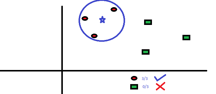
It can be used for both classification and regression problems. However, it is more widely used in classification problems in the industry. K nearest neighbors is a simple algorithm that stores all available cases and classifies new cases by a majority vote of its k neighbors. The case being assigned to the class is most common amongst its K nearest neighbors measured by a distance function.
These distance functions can be Euclidean, Manhattan, Minkowski and Hamming distance. First three functions are used for continuous function and fourth one (Hamming) for categorical variables. If K = 1, then the case is simply assigned to the class of its nearest neighbor. At times, choosing K turns out to be a challenge while performing KNN modeling.
n차원 공간에서 Input Data를 분류할때 그 가까운 주변 이웃들에게 투표권을 주어서 결정하는 방법, 몇명한테 투표권을 주는 지가 K를 결정. K=1인 경우 그냥 제일 가까운 이웃과 똑같이 분류된다.
K=1: 배우자의 흡연여부를 보고 상대방의 흡연 여부를 예측
K=2~ : 다른 가족, 친구 들에게 Voting 권한을 주어 흡연 여부를 예측
More: Introduction to k-nearest neighbors : Simplified.
KNN can easily be mapped to our real lives. If you want to learn about a person, of whom you have no information, you might like to find out about his close friends and the circles he moves in and gain access to his/her information!
Things to consider before selecting KNN:
- KNN is computationally expensive (KNN은 비싸다)
- Variables should be normalized else higher range variables can bias it 농구실력을 추정할때 키, 속도, 시력을 그냥 쓰면 안된다. 정규화 필요
- Works on pre-processing stage more before going for KNN like outlier, noise removal
Python Code
#Import Library
from sklearn.neighbors import KNeighborsClassifier
#Assumed you have, X (predictor) and Y (target) for training data set and x_test(predictor) of test_dataset
# Create KNeighbors classifier object model
KNeighborsClassifier(n_neighbors=6) # default value for n_neighbors is 5
# Train the model using the training sets and check score
model.fit(X, y)
#Predict Output
predicted= model.predict(x_test)
R Code
library(knn)
x <- cbind(x_train,y_train)
# Fitting model
fit <-knn(y_train ~ ., data = x,k=5)  # 이웃을 5명으로 지정
summary(fit)
#Predict Output
predicted= predict(fit,x_test)
