daTa-dRiveN

7. K-Means

It is a type of unsupervised algorithm which  solves the clustering problem. Its procedure follows a simple and easy  way to classify a given data set through a certain number of  clusters (assume k clusters). Data points inside a cluster are homogeneous and heterogeneous to peer groups.

Remember figuring out shapes from ink blots? k means is somewhat similar this activity. You look at the shape and spread to decipher how many different clusters / population are present!

How K-means forms cluster:

1. K-means picks k number of points for each cluster known as centroids.   (K개의 중심점을 찍는다.)
2. Each data point forms a cluster with the closest centroids i.e. k clusters.  (각 Data Point 를 중심점으로 묶는다) 
3. Finds the centroid of each cluster based on existing cluster members. Here we have new centroids. (각 cluster별로 새로운 중심점을 잡는다) 
4. As we have new centroids, repeat step 2 and 3. Find the closest distance for each data point from new centroids and get associated with new k-clusters. Repeat this process until convergence occurs i.e. centroids does not change.
   (위의 2,3번을 중심점이 변하지 않을때까지 반복한다) 

How to determine value of K:

In K-means, we have clusters and each cluster has its own centroid. Sum of square of difference between centroid and the data points within a cluster constitutes within sum of square value for that cluster. Also, when the sum of square values for all the clusters are added, it becomes total within sum of square value for the cluster solution.

중심점과 그 cluster내 datapoint 사이의 거리제곱근합은 중심점의 갯수가 늘어갈 수록 적어진다. 즉, 동일 cluster내 중심점과 유사성은 점점 커진다.

= 고객 세그먼트를 잘게 나눌수록 그 세그먼트 대표 profile(= 중심점)과 data point는 점점 유사해 진다. 

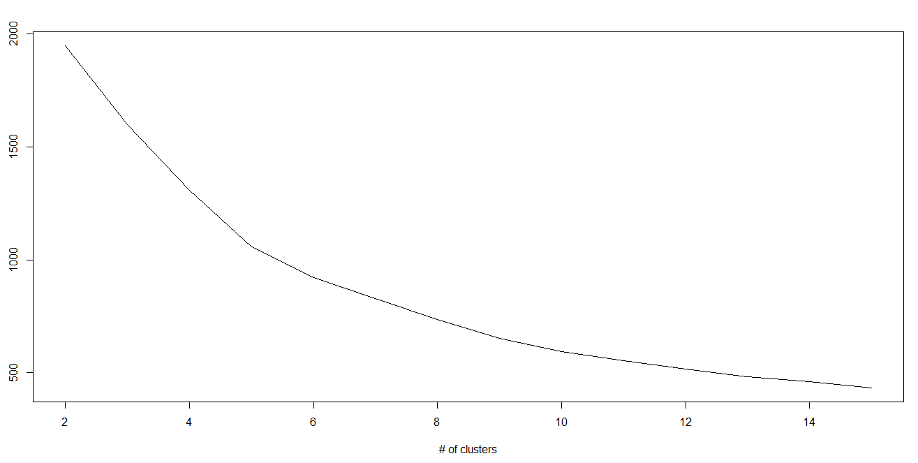
We know that as the number of cluster increases, this value keeps on decreasing but if you plot the result you may see that the sum of squared distance decreases sharply up to some value of k, and then much more slowly after that. Here, we can find the optimum number of cluster.

Python Code

#Import Library
from sklearn.cluster import KMeans
#Assumed you have, X (attributes) for training data set and x_test(attributes) of test_dataset
# Create KNeighbors classifier object model 
k_means = KMeans(n_clusters=3, random_state=0)
# Train the model using the training sets and check score
model.fit(X)
#Predict Output
predicted= model.predict(x_test)

R Code

library(cluster)
fit <- kmeans(X, 3) # 3 cluster solution # 3개의 중심점을 만들어 시작한다.

8. Random Forest 랜덤 포레스트 

Random Forest is a trademark term for an ensemble of decision trees. In Random Forest, we’ve collection of decision trees (so known as “Forest”). To classify a new object based on attributes, each tree gives a classification and we say the tree “votes” for that class. The forest chooses the classification having the most votes (over all the trees in the forest).

의사결정나무 여러개의 집합을 만들어 숲이라 부른다. 새로운 값을 분류(classification) 하고자 할때 각각의 나무에게 투표권을 주어서 가장 많은 나무로 부터 득표한 class에 할당한다. 

Each tree is planted & grown as follows:

1. If the number of cases in the training set is N, then sample of N cases is taken at random but with replacement. This sample will be the training set for growing the tree.
   훈련셋에서 일부를 복원 추출법으로 추출한다
   
   
2. If there are M input variables, a number m<<M is specified such that at each node, m variables are selected at random out of the M and the best split on these m is used to split the node. The value of m is held constant during the forest growing.
   입력변수가 모두 M개일때 그중 m개를 무작위로 뽑아서 Decision Tree만드는 방식으로 분기노드를 만든다 
3. Each tree is grown to the largest extent possible. There is no pruning.  가지치기는 없다. 
   
   

For more details on this algorithm, comparing with decision tree and tuning model parameters, I would suggest you to read these articles:

1. Introduction to Random forest – Simplified

2. Comparing a CART model to Random Forest (Part 1)

3. Comparing a Random Forest to a CART model (Part 2)

4. Tuning the parameters of your Random Forest model

Python

#Import Library
from sklearn.ensemble import RandomForestClassifier
#Assumed you have, X (predictor) and Y (target) for training data set and x_test(predictor) of test_dataset
# Create Random Forest object
model= RandomForestClassifier()
# Train the model using the training sets and check score
model.fit(X, y)
#Predict Output
predicted= model.predict(x_test)

R Code

library(randomForest)
x <- cbind(x_train,y_train)
# Fitting model
fit <- randomForest(Species ~ ., x,ntree=500)   # 트리를 500개 만든다는 뜻
summary(fit)
#Predict Output 
predicted= predict(fit,x_test)

5. Naive Bayes 나이브 베이즈 모델 

It is a classification technique based on Bayes’ theorem with an assumption of independence between predictors. In simple terms, a Naive Bayes classifier assumes that the presence of a particular feature in a class is unrelated to the presence of any other feature. For example, a fruit may be considered to be an apple if it is red, round, and about 3 inches in diameter. Even if these features depend on each other or upon the existence of the other features, a naive Bayes classifier would consider all of these properties to independently contribute to the probability that this fruit is an apple.

나이브 베이즈 모델은 입력변수가 서로 독립이라고 가정한다. 
예들들어 5년내 당뇨병 발병 가능성을 예측할 때 입력변수로 현재 몸무게, 평소운동량, 음주/흡연량, 설탕소비량을 입력값으로 쓴다고 가정해보자. 그런데 나이브 베이즈 모델은 설탕 소비량, 평소 운동량이 몸무게에 아무런 영향을 주지 않는다고 가정한다.
이름처럼 나이브한 구석이 있다.

Naive Bayesian model is easy to build and particularly useful for very large data sets. Along with simplicity, Naive Bayes is known to outperform even highly sophisticated classification methods.

대용량 데이터에 적용하기 좋고, 다른 분류(Classification) 보다 성능이 좋다. 

Bayes theorem provides a way of calculating posterior probability P(c|x) from P(c), P(x) and P(x|c). Look at the equation below:

 P(c|x) = 비만인 경우 당뇨가 될 확률 (= posterior probability) 
 P(x|c) = 당뇨인 경우 비만인 확률(=likelihood) , P(x) = 전체중 비만일 확률,  P(c) = 전체 중 당뇨인 확률(=prior probability)

 P(c|x) = 15% = 3/20  = 60% * 5% /20%

Here,

• P(c|x) is the posterior probability of class (target) given predictor (attribute). 
• P(c) is the prior probability of class. 
• P(x|c) is the likelihood which is the probability of predictor given class. 
• P(x) is the prior probability of predictor.

Example: Let’s understand it using an example. Below I have a training data set of weather and corresponding target variable ‘Play’. Now, we need to classify whether players will play or not based on weather condition. Let’s follow the below steps to perform it.

Step 1: Convert the data set to frequency table

Step 2: Create Likelihood table by finding the probabilities like Overcast probability = 0.29 and probability of playing is 0.64.

Step 3: Now, use Naive Bayesian equation to calculate the posterior probability for each class. The class with the highest posterior probability is the outcome of prediction.

Problem: Players will pay if weather is sunny, is this statement is correct?

We can solve it using above discussed method, so P(Yes | Sunny) = P( Sunny | Yes) * P(Yes) / P (Sunny)

Here we have P (Sunny |Yes) = 3/9 = 0.33, P(Sunny) = 5/14 = 0.36, P( Yes)= 9/14 = 0.64

Now, P (Yes | Sunny) = 0.33 * 0.64 / 0.36 = 0.60, which has higher probability.

위 표의 경우 3/5 = 60%하는 P(Yes/Sunny) 값이 금방 나오지만, 현실 사례에서는 그렇지 않기 때문에 Navie Bayse를 사용
Decision tree와 달리 하나의 값(Sunny)만으로도 결과(yes)확률을 알수 있다

Naive Bayes uses a similar method to predict the probability of different class based on various attributes. This algorithm is mostly used in text classification and with problems having multiple classes.
- 스팸필터와 같이 많은 변수(attributes)가 있는 경우에 활용하기 좋다. 

 Python Code

#Import Library
from sklearn.naive_bayes import GaussianNB
#Assumed you have, X (predictor) and Y (target) for training data set and x_test(predictor) of test_dataset
# Create SVM classification object model = GaussianNB() # there is other distribution for multinomial classes like Bernoulli Naive Bayes, Refer link
# Train the model using the training sets and check score
model.fit(X, y)
#Predict Output
predicted= model.predict(x_test)

R Code

library(e1071)
x <- cbind(x_train,y_train)
# Fitting model
fit <-naiveBayes(y_train ~ ., data = x)
summary(fit)
#Predict Output 
predicted= predict(fit,x_test)

6. KNN (K- Nearest Neighbors) K- 최근접 이웃

It can be used for both classification and regression problems. However, it is more widely used in classification problems in the industry. K nearest neighbors is a simple algorithm that stores all available cases and classifies new cases by a majority vote of its k neighbors. The case being assigned to the class is most common amongst its K nearest neighbors measured by a distance function.

These distance functions can be Euclidean, Manhattan, Minkowski and Hamming distance. First three functions are used for continuous function and fourth one (Hamming) for categorical variables. If K = 1, then the case is simply assigned to the class of its nearest neighbor. At times, choosing K turns out to be a challenge while performing KNN modeling.

n차원 공간에서 Input Data를 분류할때 그 가까운 주변 이웃들에게 투표권을 주어서 결정하는 방법, 몇명한테 투표권을 주는 지가 K를 결정. K=1인 경우 그냥 제일 가까운 이웃과 똑같이 분류된다. 

K=1: 배우자의 흡연여부를 보고 상대방의 흡연 여부를 예측

K=2~ :  다른 가족, 친구 들에게 Voting 권한을 주어 흡연 여부를 예측 

More: Introduction to k-nearest neighbors : Simplified.

KNN can easily be mapped to our real lives. If you want to learn about a person, of whom you have no information, you might like to find out about his close friends and the circles he moves in and gain access to his/her information!

Things to consider before selecting KNN:

• KNN is computationally expensive   (KNN은 비싸다) 
• Variables should be normalized else higher range variables can bias it  농구실력을 추정할때 키, 속도, 시력을 그냥 쓰면 안된다. 정규화 필요 
• Works on pre-processing stage more before going for KNN like outlier, noise removal

Python Code

#Import Library
from sklearn.neighbors import KNeighborsClassifier
#Assumed you have, X (predictor) and Y (target) for training data set and x_test(predictor) of test_dataset
# Create KNeighbors classifier object model 
KNeighborsClassifier(n_neighbors=6) # default value for n_neighbors is 5
# Train the model using the training sets and check score
model.fit(X, y)
#Predict Output
predicted= model.predict(x_test)

R Code

library(knn)
x <- cbind(x_train,y_train)
# Fitting model
fit <-knn(y_train ~ ., data = x,k=5)  # 이웃을 5명으로 지정 
summary(fit)
#Predict Output 
predicted= predict(fit,x_test)

3. Decision Tree : 의사 결정 나무 

This is one of my favorite algorithm and I use it quite frequently. It is a type of supervised learning algorithm that is mostly used for classification problems. Surprisingly, it works for both categorical and continuous dependent variables. In this algorithm, we split the population into two or more homogeneous sets. This is done based on most significant attributes/ independent variables to make as distinct groups as possible. For more details, you can read: Decision Tree Simplified.

source: statsexchange

입력변수가 여러개다.  (맑음, 보통, 비온다) - (습도가 높다/낮다) - (바람이 분다/안분다) 
이로부터 야구 경기를 할지 말지 예측(출력) 하는 것.  test set으로부터 어떻게 입력변수로 분기시키면 최적의 예측(classification)이 가능한지 모델을 만든다.  

In the image above, you can see that population is classified into four different groups based on multiple attributes to identify ‘if they will play or not’. To split the population into different heterogeneous groups, it uses various techniques like Gini, Information Gain, Chi-square, entropy.

어떻게 의사결정 나무가 모델링되는 지는 여러가지 방법이 있고 여기서는 몰라도 된다. 

The best way to understand how decision tree works, is to play Jezzball – a classic game from Microsoft (image below). Essentially, you have a room with moving walls and you need to create walls such that maximum area gets cleared off with out the balls.

So, every time you split the room with a wall, you are trying to create 2 different populations with in the same room. Decision trees work in very similar fashion by dividing a population in as different groups as possible.

More: Simplified Version of Decision Tree Algorithms

Python Code

#Import Library
#Import other necessary libraries like pandas, numpy...
from sklearn import tree
#Assumed you have, X (predictor) and Y (target) for training data set and x_test(predictor) of test_dataset
# Create tree object 
model = tree.DecisionTreeClassifier(criterion='gini') # for classification, here you can change the algorithm as gini or entropy (information gain) by default it is gini  
# model = tree.DecisionTreeRegressor() for regression
# Train the model using the training sets and check score
model.fit(X, y)
model.score(X, y)
#Predict Output
predicted= model.predict(x_test)

R Code

library(rpart)
x <- cbind(x_train,y_train)
# grow tree 
fit <- rpart(y_train ~ ., data = x,method="class") # 입력변수에 분기에 활용할수 있는 조건이 들어 있다 
summary(fit)
#Predict Output 
predicted= predict(fit,x_test)

4. SVM (Support Vector Machine)

It is a classification method. In this algorithm, we plot each data item as a point in n-dimensional space (where n is number of features you have) with the value of each feature being the value of a particular coordinate.

For example, if we only had two features like Height and Hair length of an individual, we’d first plot these two variables in two dimensional space where each point has two co-ordinates (these co-ordinates are known as Support Vectors)

 N차원 공간에 이미 분류된(서로 다른 색깔의) 공을 나누는 직선을 긋는 것이다. 

Now, we will find some line that splits the data between the two differently classified groups of data. This will be the line such that the distances from the closest point in each of the two groups will be farthest away.

In the example shown above, the line which splits the data into two differently classified groups is the black line, since the two closest points are the farthest apart from the line. This line is our classifier. Then, depending on where the testing data lands on either side of the line, that’s what class we can classify the new data as.

More: Simplified Version of Support Vector Machine

Think of this algorithm as playing JezzBall in n-dimensional space. The tweaks in the game are:

• You can draw lines / planes at any angles (rather than just horizontal or vertical as in classic game)
• The objective of the game is to segregate balls of different colors in different rooms.
• And the balls are not moving.

Python Code

#Import Library
from sklearn import svm
#Assumed you have, X (predictor) and Y (target) for training data set and x_test(predictor) of test_dataset
# Create SVM classification object 
model = svm.svc() # there is various option associated with it, this is simple for classification. You can refer link, for mo# re detail.
# Train the model using the training sets and check score
model.fit(X, y)
model.score(X, y)
#Predict Output
predicted= model.predict(x_test)

R Code

library(e1071)
x <- cbind(x_train,y_train)
# Fitting model
fit <-svm(y_train ~ ., data = x)
summary(fit)
#Predict Output 
predicted= predict(fit,x_test)

1. Linear Regression

It is used to estimate real values (cost of houses, number of calls, total sales etc.) based on continuous variable(s). Here, we establish relationship between independent and dependent variables by fitting a best line. This best fit line is known as regression line and represented by a linear equation Y= a *X + b.

The best way to understand linear regression is to relive this experience of childhood. Let us say, you ask a child in fifth grade to arrange people in his class by increasing order of weight, without asking them their weights! What do you think the child will do? He / she would likely look (visually analyze) at the height and build of people and arrange them using a combination of these visible parameters. This is linear regression in real life! The child has actually figured out that height and build would be correlated to the weight by a relationship, which looks like the equation above.

초등학교 키(입력), 몸무게(목표) Data가 있다. 여기서 키만 가지고 몸무게를 추정하는 1차 함수를 만들고, 이의 결과 예측 수준을 최대로 높인다.   이로써 키만가지고 몸무게를 예측할수 있게 된다. 여기서 입력이 늘어나면 Multiple되고, Curvilinear도 될수 있다. 

In this equation:

• Y – Dependent Variable
• a – Slope
• X – Independent variable
• b – Intercept

These coefficients a and b are derived based on minimizing the sum of squared difference of distance between data points and regression line.

Look at the below example. Here we have identified the best fit line having linear equationy=0.2811x+13.9. Now using this equation, we can find the weight, knowing the height of a person.

Linear Regression is of mainly two types: Simple Linear Regression and Multiple Linear Regression. Simple Linear Regression is characterized by one independent variable. And, Multiple Linear Regression(as the name suggests) is characterized by multiple (more than 1) independent variables. While finding best fit line, you can fit a polynomial(다항) or curvilinear(곡선) regression. And these are known as polynomial or curvilinear regression.

Python Code

#Import Library
#Import other necessary libraries like pandas, numpy...
from sklearn import linear_model
#Load Train and Test datasets
#Identify feature and response variable(s) and values must be numeric and numpy arrays
x_train=input_variables_values_training_datasets
y_train=target_variables_values_training_datasets
x_test=input_variables_values_test_datasets
# Create linear regression object
linear = linear_model.LinearRegression()
# Train the model using the training sets and check score
linear.fit(x_train, y_train)
linear.score(x_train, y_train)
#Equation coefficient and Intercept
print('Coefficient: \n', linear.coef_)
print('Intercept: \n', linear.intercept_)
#Predict Output
predicted= linear.predict(x_test)

R Code

#Load Train and Test datasets
#Identify feature and response variable(s) and values must be numeric and numpy arrays
x_train <- input_variables_values_training_datasets ## (훈련, 몸무게 입력치) 
y_train <- target_variables_values_training_datasets ## (훈련, 키 목표치)
x_test <- input_variables_values_test_datasets ## (테스트, 몸무게 입력치) 
x <- cbind(x_train,y_train)  ## 훈련셋으로 묶는다
# Train the model using the training sets and check score
linear <- lm(y_train ~ ., data = x)  ## x셋으로부터 목표치(몸무게)를 만드는 회귀모델을 만드다. 
summary(linear)        ## 만들어진 회수함수를 요약해서 보여준다. 
#Predict Output         
predicted= predict(linear,x_test) ## 테스트 입력치를 통해 목표치를 출력한다.  

 

2. Logistic Regression

Don’t get confused by its name! It is a classification not a regression algorithm. It is used to estimate discrete values ( Binary values like 0/1, yes/no, true/false ) based on given set of independent variable(s). In simple words, it predicts the probability of occurrence of an event by fitting data to a logit function. Hence, it is also known as logit regression. Since, it predicts the probability, its output values lies between 0 and 1 (as expected).

회권분석같지만 사실상 classification(분류)다. 입력- 출력에서 출력은 yes/no에 대한 확률값으로 나타난다.
키를 입력값으로 농구부에 입단할 가능성을 출력값으로 한다.  

Again, let us try and understand this through a simple example.

Let’s say your friend gives you a puzzle to solve. There are only 2 outcome scenarios – either you solve it or you don’t. Now imagine, that you are being given wide range of puzzles / quizzes in an attempt to understand which subjects you are good at. The outcome to this study would be something like this – if you are given a trignometry based tenth grade problem, you are 70% likely to solve it. On the other hand, if it is grade fifth history question, the probability of getting an answer is only 30%. This is what Logistic Regression provides you.

입력: 고2 미적분  --> 출력: 풀수 있는 확률 25% 
입력: 중2 인수분해 --> 출력: 풀수 있는 확률 85%

Coming to the math, the log odds of the outcome is modeled as a linear combination of the predictor variables.

odds= p/ (1-p) = probability of event occurrence / probability of not e. occur. p=70% --> 233.3% 
ln(odds) = ln(p/(1-p))
logit(p) = ln(p/(1-p)) = b0+b1X1+b2X2+b3X3....+bkXk

Above, p is the probability of presence of the characteristic of interest. It chooses parameters that maximize the likelihood of observing the sample values rather than that minimize the sum of squared errors (like in ordinary regression).

로지스틱스 회귀 모델은 S.E.의 sum을 줄이기 보다는 결과를 맞출 확률을 최대화하는 쪽으로 변수를 선택한다. 

Now, you may ask, why take a log? For the sake of simplicity, let’s just say that this is one of the best mathematical way to replicate a step function. I can go in more details, but that will beat the purpose of this article.

로그값을 쓰는 이유는 이것이 Step Function(계단식 함수) 을 모사하기에 가장 좋은 방법이기 때문이다.  아마도 가운데 grey한 구간이 아닌 양쪽끝 (0 또는 1)에 값이 몰리기 때문으로 보임 

Python Code

#Import Library
from sklearn.linear_model import LogisticRegression
#Assumed you have, X (predictor) and Y (target) for training data set and x_test(predictor) of test_dataset
# Create logistic regression object
model = LogisticRegression()
# Train the model using the training sets and check score
model.fit(X, y)
model.score(X, y)
#Equation coefficient and Intercept
print('Coefficient: \n', model.coef_)
print('Intercept: \n', model.intercept_)
#Predict Output
predicted= model.predict(x_test)

R Code

x <- cbind(x_train,y_train)
# Train the model using the training sets and check score
logistic <- glm(y_train ~ ., data = x,family='binomial') # x학습셋으로부터 결과값인 확률(y)를 추정할수 있는 
summary(logistic)                                        # 함수를 만든다. 
#Predict Output
predicted= predict(logistic,x_test)

 

Furthermore..

There are many different steps that could be tried in order to improve the model:

• including interaction terms
• removing features
• regularization techniques
• using a non-linear model

#1. 

We are probably living in the most defining period of human history. The period when computing moved from large mainframes to PCs to cloud. But what makes it defining is not what has happened, but what is coming our way in years to come.

What makes this period exciting for some one like me is the democratization of the tools and techniques, which followed the boost in computing. Today, as a data scientist, I can build data crunching machines with complex algorithms for a few dollors per hour. But, reaching here wasn’t easy! I had my dark days and nights.

Who can benefit the most from this guide?

What I am giving out today is probably the most valuable guide, I have ever created.

The idea behind creating this guide is to simplify the journey of aspiring data scientists and machine learning enthusiasts across the world. Through this guide, I will enable you to work on machine learning problems and gain from experience. I am providing a high level understanding about various machine learning algorithms along with R & Python codes to run them. These should be sufficient to get your hands dirty.

I have deliberately skipped the statistics behind these techniques, as you don’t need to understand them at the start. So, if you are looking for statistical understanding of these algorithms, you should look elsewhere. But, if you are looking to equip yourself to start building machine learning project, you are in for a treat.

Broadly, there are 3 types of Machine Learning Algorithms..

1. Supervised Learning: 지도 학습 

How it works: This algorithm consist of a target / outcome variable (or dependent variable) which is to be predicted from a given set of predictors (independent variables). Using these set of variables, we generate a function that map inputs to desired outputs. The training process continues until the model achieves a desired level of accuracy on the training data. Examples of Supervised Learning: Regression, Decision Tree, Random Forest, KNN, Logistic Regression etc.

문제와 답지를 이미 가지고 있다. 이를 통해 함수를 만들어서 원하는 수준의 정확도를 나타낼때 까지 반복한다.  

2. Unsupervised Learning: 비지도 학습 

How it works: In this algorithm, we do not have any target or outcome variable to predict / estimate.  It is used for clustering population in different groups, which is widely used for segmenting customers in different groups for specific intervention. Examples of Unsupervised Learning: Apriori algorithm, K-means.

답지 없이 문제만 있다. 문제를 clustering하면서 답지를 유추한다.  정답을 볼 기회가 없다. 

3. Reinforcement Learning: 강화 학습 

How it works:  Using this algorithm, the machine is trained to make specific decisions. It works this way: the machine is exposed to an environment where it trains itself continually using trial and error. This machine learns from past experience and tries to capture the best possible knowledge to make accurate business decisions. Example of Reinforcement Learning: Markov Decision Process

오목 두는 방법을 가르치지 않고, 승패만 이야기해 준다. 수많은 시행 착오를 통해 스스로 오목의 rule을 배우도록한다. 

List of Common Machine Learning Algorithms

Here is the list of commonly used machine learning algorithms. These algorithms can be applied to almost any data problem:

1. Linear Regression
2. Logistic Regression
3. Decision Tree
4. SVM
5. Naive Bayes
6. KNN
7. K-Means
8. Random Forest
9. Dimensionality Reduction Algorithms
10. Gradient Boost & Adaboost